Everyone is hyping up GPT-4, and it’s true that it’s currently the best publicly available model. However, numerous open-source models are available that, when well utilized, can perform impressively using significantly fewer resources than GPT-4 (which is actually rumored to be a combination of eight models).
Recently, I completed a ‘talk to your document’ project for a client. There’s no shortage of startups doing this, but this client had an extra security and privacy requirement – their data could not leave their network. Thus, all processing had to happen on-premise. I informed them upfront that the inability to use GPT-4 might result in less accurate results, but they were willing to make that trade-off.
To my surprise, some open-source models proved to be extremely effective for this use case. Specifically, I created the embeddings using DistilBERT models trained on the MS Marco dataset, with FastChat-T5 as a Language Model (LM) for formulating answers.
The resulting system performed exceptionally well. The client was delighted with the performance, and importantly, the entire setup remained on-premise with no data leaving their infrastructure. Also, I was very pleasantly surprised by FastChat, which is a 3 Billion parameter model, but still answers very coherently, while being fast enough to run on a (beefy) CPU only instance!
While GPT-4 is a remarkable model, for companies with high security requirements, there exist various viable alternatives. Despite different trade-offs, these models can still provide excellent performance across a variety of tasks, and I can help you navigate those tradeoffs.
Reach out to me if you would like to have a private and secure “talk to your document” style app for your company!
BERT1Bidirectional Encoder Representations (and it’s numerous variants) models have taken the natural language processing field by storm ever since they came out and have been used to establish state of the art results in pretty much all imaginable tasks, including text analysis.
I am a Christian, so the Bible is important to me. So, I became curious to see what BERT would “think” about the Bible. The manuscripts of the Bible on which modern translations are based were written in Hebrew (Old Testament) and Greek (New Testament). There are many difficult challenges in the translation, resulting in many debates about the meaning of some words. I will conduct two experiments on the text of the New Testament to see what BERT outputs about the various forms of “love” and about the distinction between “soul” and “spirit”.
Quick BERT primer
There are many good explanations of how BERTworks and how it’s trained, so I won’t go into that, I just want to highlight two facts about it:
one of the main tasks that is used to train a BERT model is to predict a word2actually a byte pair encoded token given it’s context: “Today is a [MASK] day”. In this case it would have to predict the fourth word and possible options are “beautiful”, “rainy”, “sad” and so on.
one of the things that BERT does really well is to create contextual word embeddings. Word embeddings are mathematical representations of words, more precisely they are high dimensional vectors (768 in the case of BERT), that have a sort of semantic meaning. What this means is that the word embedding similar words is close to each other, for example, the embeddings for “king”, “queen” and “prince” would be close to each other, because they are all related to royalty, even though they have no common lemma. The contextual part means there is no one fixed word embedding for a given word (such as older models like word2vec or GloVe had), but it depends on the sentence where the word is used, so the word embedding for “bank” is different in the sentence “I am going to the bank to deposit some money” than in the sentence “He is sitting on the river bank fishing”, because they refer to different concepts (financial institution versus piece of land).
Obtaining the embeddings
Reading the data
First, let’s read the Bible in Python. I’ve used the American King James Version translation, because it uses modern words and it’s available in an easy to parse text file, where the verse number (Matthew 15:1) is separated from the text of the verse by a tab (\t):
Genesis 1:1 In the beginning God created the heaven and the earth.
verses = {}
with open('akjv.txt', 'r', encoding='utf8') as f:
    lines = f.readlines()
    for line in lines[23146:]:   # The New Testament starts at line 23146
        citation, raw_sentence = line.strip().split('\t')
        verses[citation] = raw_sentence
The next thing we need is the Strong’s numbers, which are a code for each Greek word (or rather base lemma) that appears in the New Testament. I have found a mapping to tell me the corresponding Strong’s number for (most) English words only for the ESV3I had to rename the New Testament book names and convert the file to UTF8 without BOM translation, which might mean that there are slight differences in verse boundaries, but I don’t think that the words I’m going to be analyzing will be different. Here the format is also verse number, followed by xx=<yyyy> pairs, where xx is the ordinal number for a word in the ESV translation and yyyy is the corresponding Strong’s number.
Matthew 1:1 02=<0976> 05=<1078> 07=<2424> 08=<5547> 10=<5207> 12=<1138> 14=<5207> 16=<0011>
This line says that in Matthew 1:1 the second word in the ESV translation corresponds to the Greek word with Strong’s number 976, the fifth word in English to the word with Strong’s number 1078 and so on. The Strong’s numbers are nicely preformatted into 4 character strings, so we check if a Strong’s number is in a verse by simply looking if the number is in this string, without having to parse each verse.
strongs_tags = {}
with open("esv_tags.txt") as f:
    lines = f.readlines()
    for line in lines:
        verse, strongs = line.split("\t", maxsplit=1)
        strongs_tags[verse] = strongs
Getting the embedding for a word with BERT
Let’s load the BERT model and it’s corresponding tokenizer, using the HuggingFace library:
from transformers import AutoTokenizer, AutoModel

tokenizer = AutoTokenizer.from_pretrained('bert-base-cased')
model = model = AutoModel.from_pretrained('bert-base-cased', output_hidden_states=True).eval()
BERT has a separate tokenizer because it doesn’t work on characters or on words directly, but it works on byte pair encoded tokens. For more frequent words, there is a 1:1 mapping of word – token, but rarer words (or words with typos) will be split up into multiple tokens. Let’s see this for the word “love” and for “aardvark”:
[CLS] and [SEP] are two special tokens, mostly relevant during training. The word_ids function returns the index of the word to which that token belongs. Let’s see an example with a rare word:
In this case, aardvarks (the second word) is split up into 4 tokens, which is why it shows up 4 times in the list obtained from word_ids.
Now, let’s find the index of the word we are looking for in a verse:
def get_word_idx(sent: str,  word: str):
    l = re.split('([ .,!?:;""()\'-])', sent)
    l = [x for x in l if x != " " and x != ""]
    return l.index(word)
We split on punctuation and spaces, skip empty strings and ones with a space and get the index of the word we are looking for.
Because the BPE encoding can give multiple tokens for one word, we have to get all the tokens that correspond to it:
encoded = tokenizer.encode_plus(sent, return_tensors="pt")

idx = get_word_idx(sent, word)
# get all token idxs that belong to the word of interest
token_ids_word = np.where(np.array(encoded.word_ids()) == idx)
In BERT, the best word embeddings have been obtained by taking the sum of the last 4 layers. We pass the encoded sentence through the model to get the outputs at the last 4 ones, sum them up layerwise and then average the outputs corresponding to the tokens that are part of our word:
def get_embedding(tokenizer, model, sent, word, layers=None):
    layers = [-4, -3, -2, -1] if layers is None else layers

    encoded = tokenizer.encode_plus(sent, return_tensors="pt")

    idx = get_word_idx(sent, word)
    # get all token idxs that belong to the word of interest
    token_ids_word = np.where(np.array(encoded.word_ids()) == idx)

    with torch.no_grad():
        output = model(**encoded)

    # Get all hidden states
    states = output.hidden_states
    # Stack and sum all requested layers
    output = torch.stack([states[i] for i in layers]).sum(0).squeeze()
    # Only select the tokens that constitute the requested word
    word_tokens_output = output[token_ids_word]

    return word_tokens_output.mean(dim=0)
Processing the New Testament with BERT
Now let’s get the embeddings for the target words from all the verses of the New Testament. We will go through all the verses and if any of the Strong’s numbers appear in the verse, we will start looking for a variation of the target word in English and get the embedding for it. The embedding, the verse text, the Greek word and the book where it appears will be appended to a list.
def get_all_embeddings(greek_words, english_words):
    embeddings = []

    for key, t in verses.items():
        strongs = strongs_tags[key]
        for word in greek_words:
            for number in greek_words[word]:
                if number in strongs:
                    gw = word

                    for v in english_words:
                        try:
                            if v in t:
                                emb = get_embedding(tokenizer, model, t, v).numpy()
                                book = books.index(key[:key.index(" ", 4)])
                                embeddings.append((emb, f"{key} {t}",  gw, book))
                                break
                        except ValueError as e:
                            print("Embedding not found", t)
                    else:
                        print("English word not found", key, t)
    return embeddings
Next, I am going to take all the verses where one of these target words appear in the New Testament. I am going to mask out their appearance and ask BERT to predict what word should be there.
def mask_and_predict(word_list):
    predictions = []
    for key, t in verses.items():
        for v in word_list:
                if v in t:
                    try:
                        new_t = re.sub(f"\\b{v}\\b", "[MASK]", t)
                        top_preds = unmasker(new_t)
                        if type(top_preds[0]) == list:
                            top_preds = top_preds[0]
                        predictions.append((f"{key} {t}",  v, top_preds))
                        break
                    except Exception:
                        print(new_t, v)
    return predictions
Love
In Greek, there are several words that are commonly translated as love: agape, eros, philia, storge, philautia, xenia, each having a different focus/source. In the New Testament, two of these are used: agape and philia. There is much debate between Christians about the exact meaning of these two words, such as whether agape is bigger than philia, the two are mostly synonyms, or philia is the bigger love.
To try to understand what BERT thinks about these two variants, I am going to extract the 768 dimensional word embeddings for the English word love, reduce their dimensionality with UMAP and plot the results, color coding them by the original word used in Greek.
Now we’ll need the Strong’s numbers for the two words we’re investigating. I included several variations for each word, such as verbs/nouns, or composite variants, such as 5365 – philarguria, which is philos + arguria, meaning love of money.
There are some weird failure cases: in 1 Corinthians 13, famously called the chapter of love, the AKJV uses charity for example instead of love for the Greek word “agape”. I chose to not look for charity as well, so all those uses of “agape” are left out.
Now that we have all the embeddings, let’s reduce their dimensionality with UMAP and then visualize them. They will be color coded according to the Greek word and on hover they will show the verse.
The blue dots are where the Greek is agape (or it’s derivatives), while the red ones are where the Greek is philos.
You can notice 4 clusters in the data. The top right cluster is mostly made out of love that is between Christians. The bottom right one seems to be mostly about the love of God, with the love of money throw in there as well (the blue dot on the right). The cluster on the left seems to be less well defined, with the top side looking like it’s about commandments related to love (you shall love, should love, if anyone will love) and it’s consequences. The bottom left side is the most fuzzy, but I think it seems to be about the practical love of Jesus for humans.
What is easier to notice is that the Greek words agape and philos are mixed together. The love of God cluster (bottom right) seems to be the only one that is agape only (if we exclude the love of money verse, which reeaaaally doesn’t belong with the others), with the exception of the Titus 3:4 verse, which however does sound very much like the others.
However, we can plot the same graph, but this time color coding with the parts of the New Testament where the verse is found:
There is lots of mixing in all clusters, but it seems to me that the Pauline letters use love in a different way then the gospels.
Conclusion? Yes, the word agape does sometimes refer to the love of God, in a seemingly special way, but it often refers to other kinds of love as well, in a way which BERT can’t really distinguish from philos love.
Soul and spirit
The Bible uses two words for the immaterial parts of man: soul (Hebrew: nephesh, Greek: psuche) and spirit (Hebrew: ruach, Greek: pneuma). Again, there is great debate whether the two are used interchangeably or whether they are two distinct components of humans.
After getting the embeddings for these two words, I will plot them as we did before. We can discover quite a few clusters in this way.
In this case, the clusters are almost perfectly separated, with very little mixing. What little mixing happens is usually because in one verse both words occur. Contrast this with the case for agape/phileo, where there is a lot of mixing.
The top right cluster is about the Spirit of God. The one below is about unclean/evil spirits. The middle cluster is about the Holy Spirit. The bottom left cluster is mostly about the spirit of man, with some examples from the other clusters.
The interesting thing is that the two verses used as most common arguments for the soul being distinct from the spirit (1 Thessalonians 5:23 and Hebrews 4:12) are placed in the blue cluster, and they are right next to Matthew 22:37, Mark 12:30 and Luke 10:27, verses which indicate that man is made of different components (heart, soul, mind, strength).
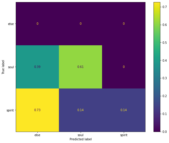
Now, let’s mask out the words soul and spirit and ask BERT to predict the missing word. If BERT mixes the two half the time, it means it thinks there is no distinction between them. Otherwise, they are probably distinct. The resulting confusion matrix:
The y axis represent the true word (soul or spirit), the x axis represents the predicted word (something else, soul or spirit). We can see that in more that 60% of the cases it predicts soul correctly. It never mispredicts it to spirit, but in 40% of the cases it does predict something else. For spirit, the results are worse: it predicts something else quite often, and on top of that, it predicts 50-50% between soul and spirit, so it mixes them up quite often.
The conclusion? The evidence is mixed: on one hand, usages of soul and spirit seem to be mostly different, because they cluster very neatly. But some key verses for the distinction are put in the soul cluster. Now, this might happen because of the way BERT extracts embeddings, two words that are in the same sentence will have similar embeddings. On the other hand, because of the way spirit is mispredicted, it would seem to indicate that there is significant overlap between spirit and soul, at least as “understood” by BERT.
Conclusion
I believe with some polish, BERT-style models can eventually make their way into the toolbox of someone who studies the Bible. They can offer a more consistent perspective to analyzing the text. And of course, they can be used not just to analyze the Bible, but for many other purposes, such as building tools for thoughts (using computers to help us think better and faster), or to analyze all kinds of documents, to cluster them, to extract information from them or to categorize them.
If you need help with that, feel free to reach out to me.
The full code for this analysis can be found in this Colab.
Data is crucial to any machine learning effort. And not just any data, but annotated data, so that the machine learning algorithms can learn what is the outcome it should predict. In some cases, we can get the data from some existing processes in the business, but more often than not, we need to set up a manual annotation process.
For annotating freeform text data (text generated by people) there is a great open source tool called Doccano. It is used to gather data for a wide range of common natural language processing (NLP) tasks, such as sentiment analysis, document classification, named entity recognition (NER), summarization, question answering, translation and others.
Text Annotation types
There are three kinds of data annotation types in Doccano.
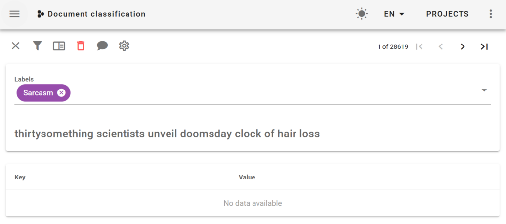
Text classification
This kind of project enables you to annotate labels that apply to the entire document. For example, in a sentiment analysis task, you could label a document as being positive or negative. In a document classification task you will annotate what’s the topic of the document. You can choose multiple labels for each document.
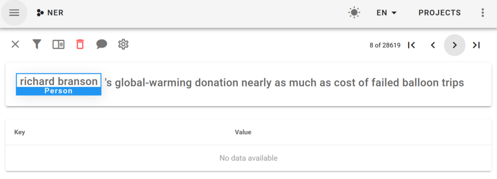
Sequence Labeling
This is generally used for NER tasks, where you select relevant fragments from the text. For example, where are persons or organizations mentioned in documents. There can be several fragments selected for each document.
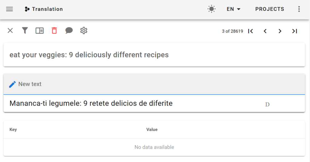
Sequence to Sequence
The Seq2seq annotation is for tasks such as summarization, question answering or translations from one language to another. There is a text box where you can write the appropriate response. For summarization, this would be the summary of the document. For questions, you can write several answers.
Setting up Doccano
Doccano offers 1-click installs for AWS, Azure and Heroku, or you can run it locally using Docker.
After you have Doccano running, you must create a new project and import your documents. Doccano is quite flexible and you can import data in multiple formats, such as plain text, CSV, JSONL or even fastText format.
You can create multiple users who will work on annotation. They can review each others work or they can annotate independently each document. In this case, the annotations from different labelers can be compared. If there are big differences, maybe the task is not clear and better guidelines are needed – if humans can’t solve the problem, machine learning won’t be able to solve it either.
Doccano features
Doccano is trying to make the annotation workflow as efficient as possible by giving keyboard shortcuts for most actions.
It has a dashboard where you can see statistics about how many documents were annotated, what’s the frequency of labels and how many documents were processed by each labeler.
You can also speed up the process by using an existing machine learning model to bootstrap the annotations. Either when uploading the data you specify some existing labels or you can configure Docanno to make a call to another REST API and get annotations from there. Then the labelers only have to review the output of the algorithm, instead of annotating from scratch.
Text Annotation Alternatives
There are other annotation tools as well. One for example is Prodigy, from the makers of Spacy, one of the most popular NLP libraries. It has a tight integration with Spacy and it has support for active learning, but it’s a paid product, unlike Doccano.
Another option is Label Studio, which supports annotating images, audio and time series, not just text.
If you need help setting up a text annotation pipeline to make sure that you are gathering the right data for your problem, don’t hesitate to contact me.
Machine learning (ML) has exploded in the last decade. Most companies try to apply ML in all kinds of areas, from image processing problems (such as recognizing defects in manufacturing), to forecasting, to trying to extract meaning from unstructured text, and many other problems. A quite common task is that of trying to classify documents into various classes. For example, you have many news articles and you want to group them by their topics, such as politics, entertainment, health, sports and travel. Another example would be a company that has many documents and wants to classify them by their type: invoices, resumes, various reports, and so on.
One of the big challenges of machine learning is that it requires a lot of annotated data. It’s not enough to just get a lot of news articles, a human has to go and annotate at least several thousands of them with their topic and only then can you start applying ML algorithms to solve your problem. In general, the more annotated data points you have, the better accuracy you get.
But getting the data is time-consuming and expensive. In some cases, you can crowdsource the data gathering, using a service such as Mechanical Turk, but in other cases, where more business domain knowledge is needed, the data annotation has to happen in house. If reading and classifying a document takes one minute, then annotating ten thousand documents will take 160 hours, so a month of full time work for someone. To ensure that your labels are accurate, because even human labelers make mistakes, the documents should be labeled by at least three humans. So the costs quickly go up.
SentenceBERT to the rescue
Recent developments in Natural Language Processing (NLP) research have led to the creation of neural networks that have a good understanding of language out of the box. One of them in particular can be used, with a clever reframing of the problem, to solve, or at least make it easier, our problem of text classification.
SentenceBERT is a followup to BERT, making it better by using siamese networks, and is used to generate sentence embeddings. None of this makes any sense? No problem, you don’t need to understand it to get started with it, but I’ll still try to explain the gist of it.
(For some reason, many models in NLP are named after Sesame Street characters: ELMo, BERT, Rosita, ERNIE, Grover, KERMIT, Big BIRD 😄)
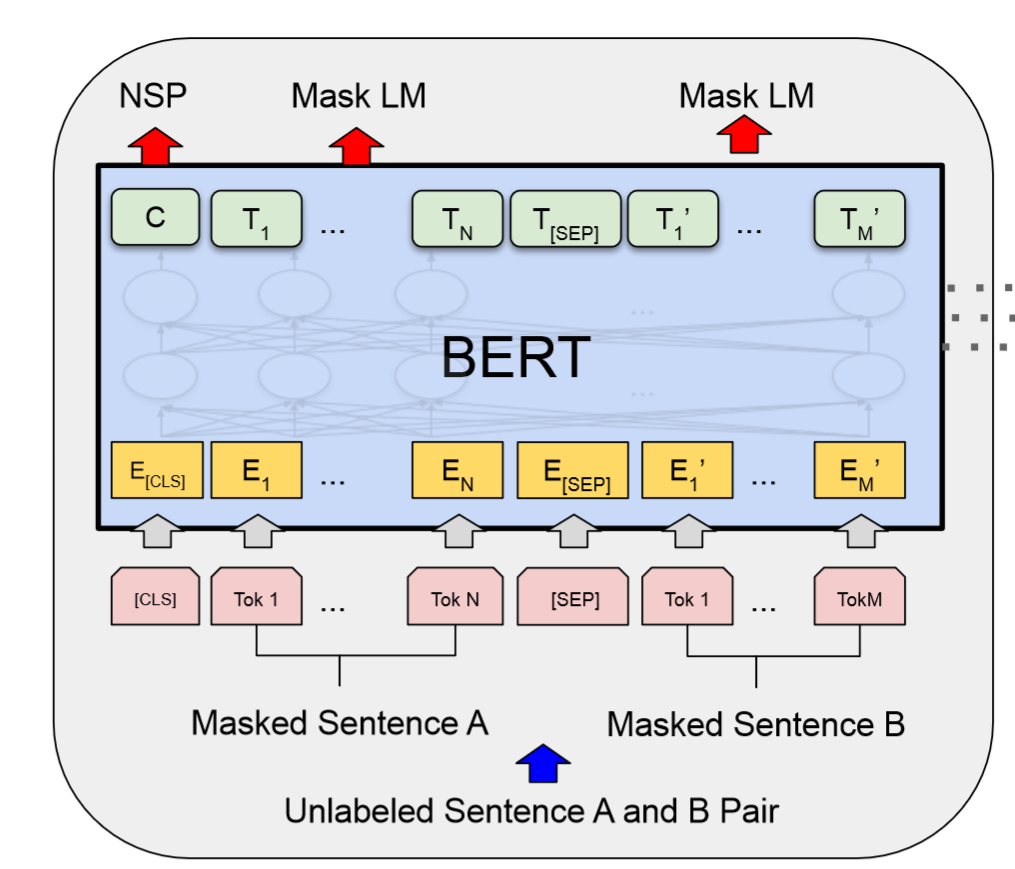
Figure 1: BERT model
The problem SentenceBERT is trained to solve is Natural Language Inference (NLI), which consists of having two sentences, a premise and a hypothesis, and the model has to say what’s the relationship between those two sentences. Does the premise entail the hypothesis, are they neutral (unrelated) or are they contradictory? For example “A soccer game with multiple males playing.” entails “Some men are playing a sport.”, but “A man inspects the uniform of a figure in some East Asian country.” contradicts “The man is sleeping.”.
A side effect of trying to solve this problem is that SentenceBERT learns to “understand” sentences quite well. Understanding sentences is quite a philosophical debate, but what I mean by this is that it reduces a sentence (or even a paragraph) to a vector of numbers, such that sentences that are similar in meaning to each other have similar vectors assigned to them. These vectors are called embeddings and then can enable us to compare sentences.
How does this help us? Remember, we wanted to do text classification of single documents, not to figure out the relationship between two documents. Well, some clever researchers from the University of Pennsylvania have found a clever way to reframe one problem into the other.
Let’s say you want to classify news articles into topics such as politics, entertainment, health, sports, and travel. You take each topic and construct a sentence like “This text is about politics”. Now, this is a NLI problem: does the article entail our artificial sentence, which contains our topic?
It’s a very simple and incredible idea, but it turns out quite well in practice.
Let’s put it into practice
We are going to use the Transformer library from an awesome company called HuggingFace 🤗. They provide a pipeline that does all this for us, so it’s quite simple to use in 6 lines:
from transformers import pipeline

classifier = pipeline("zero-shot-classification", device=0)

sequence = "Who are you voting for in 2020?"

candidate_labels = ["politics", "public health", "economics"]

result = classifier(sequence, candidate_labels)
print(result)
And the output is:
{'labels': ['politics', 'economics', 'public health'],

 'scores': [0.972518801689148, 0.014584126882255077, 0.012897057458758354],

 'sequence': 'Who are you voting for in 2020?'}
In this simple example, the question “Who are you voting for in 2020?” was classified as being about politics with 97% probability, economics 1.4% probability, and public health as 1.2% probability, so it got this example correctly.
Running this requires a GPU and having all the libraries installed. It’s not hard to set up everything on your own computer, but it works better out of the box on Colab, a free environment Google provides for running Python notebooks in the cloud. You can even request to use a GPU in Colab. A more detailed notebook about this can be found here.
If you want to try it out even simpler, without having to mess around with notebooks, HuggingFace offers a demo on their website, where you just paste in different texts and the list of labels and it classifies them for you.
Other languages
All I presented above was for texts in English. But the same approach can work for other languages as well! There are pretrained models that are tuned for other languages, such as the xlm-roberta-large-xnli. This model supports 100 different languages, including Romanian. In general, results are best in the English language, because that’s where most of the data is (The XLM Roberta model was trained on 300 GB of English texts) and where most of the research has been focused, but even for Romanian language there is a dataset of 60Gb for training, so that should be enough getting things started.
When to use this
As I mentioned before, this is best run on GPUs. You can run it on CPUs, but it will be much slower (10-20 times slower). The more labels you have, the slower it is. It’s a quite complicated model, so it takes a lot of resources.
For text classification, there are many other models that are simpler, faster, and cheaper to run. But they have the disadvantage of requiring annotated data. If you have it, try to use those.
But if for example you are prototyping an idea for a startup and you don’t have annotated data yet, this approach is very good to get you started. In the beginning, you will not have many documents to classify anyway, so the fact that it’s slower is not too problematic, and it will help you quickly validate your idea. If it works, you can then invest in gathering annotated data and then switch to a simpler model.
Another way this model can help is by bootstrapping the annotation process. You have a large set of documents without labels, you run this model over them to generate labels, which might have only 50% accuracy. Then the human labelers only have to verify the suggested labels, thus speeding up the annotation process.
Conclusion
6 years ago, computer vision had it’s so-called “ImageNet” moment, when the challenge of labeling objects in images was “solved”. A new model was presented then which blew away all previous models. NLP is now getting closer to such a moment, with models such as SentenceBERT. In this article, I presented only how to use them for text classification, but they have many other use cases, such as finding similar articles, paraphrase mining, and so on.