Everyone is hyping up GPT-4, and it’s true that it’s currently the best publicly available model. However, numerous open-source models are available that, when well utilized, can perform impressively using significantly fewer resources than GPT-4 (which is actually rumored to be a combination of eight models).
Recently, I completed a ‘talk to your document’ project for a client. There’s no shortage of startups doing this, but this client had an extra security and privacy requirement – their data could not leave their network. Thus, all processing had to happen on-premise. I informed them upfront that the inability to use GPT-4 might result in less accurate results, but they were willing to make that trade-off.
To my surprise, some open-source models proved to be extremely effective for this use case. Specifically, I created the embeddings using DistilBERT models trained on the MS Marco dataset, with FastChat-T5 as a Language Model (LM) for formulating answers.
The resulting system performed exceptionally well. The client was delighted with the performance, and importantly, the entire setup remained on-premise with no data leaving their infrastructure. Also, I was very pleasantly surprised by FastChat, which is a 3 Billion parameter model, but still answers very coherently, while being fast enough to run on a (beefy) CPU only instance!
While GPT-4 is a remarkable model, for companies with high security requirements, there exist various viable alternatives. Despite different trade-offs, these models can still provide excellent performance across a variety of tasks, and I can help you navigate those tradeoffs.
Reach out to me if you would like to have a private and secure “talk to your document” style app for your company!
Let’s take a look at how to do multi label text classification with Spacy. In multi label text classification each text document can have zero, one or more labels associated with it. This makes the problem more difficult than regular multi-class classification, both from a learning perspective, but also from an evaluation perspective. Spacy offers some tools to make that easy.
spaCy
Spacy is a great general purpose NLP library, that can be used out of the box for things like part of speech tagging, named entity recognition, dependency parsing, morphological analysis and so on. Besides the built-in modules, it can also be used to train custom models, for example for text classification.
Spacy is quite powerful out of the box, but the documentation is often lacking and there are some gotchas that can prevent a model from training, so below I am writing a simple guide to train a simple multi label text classification model with this library.
Training data format
Spacy requires training data to be in its own binary data format, so the first step will be to transform our data into this format. I will be working with the lex_glue/ecthr_a dataset in this example.
First, we have to load the dataset.
from datasets import load_dataset

dataset = load_dataset("lex_glue", 'ecthr_a')
print(dataset)
print(dataset['train'][0])
Which will output the following:
DatasetDict({
    train: Dataset({
        features: ['text', 'labels'],
        num_rows: 9000
    })
    test: Dataset({
        features: ['text', 'labels'],
        num_rows: 1000
    })
    validation: Dataset({
        features: ['text', 'labels'],
        num_rows: 1000
    })
})
{'text': ['11.  At the beginning of the events relevant to the application, K. had a daughter, P., and a son, M., born in 1986 and 1988 respectively. P.’s father is X and M.’s father is V. From March to May 1989 K. was voluntarily hospitalised for about three months, having been diagnosed as suffering from schizophrenia. From August to November 1989 and from December 1989 to March 1990, she was again hospitalised for periods of about three months on account of this illness. In 1991 she was hospitalised for less than a week, diagnosed as suffering from an atypical and undefinable psychosis. It appears that social welfare and health authorities have been in contact with the family since 1989.',
  '12.  The applicants initially cohabited from the summer of 1991 to July 1993. In 1991 both P. and M. were living with them. From 1991 to 1993 K. and X were involved in a custody and access dispute concerning P. In May 1992 a residence order was made transferring custody of P. to X.',
  ....
  '93.  J. and M.’s foster mother died in May 2001.'],
 'labels': [4]}
The dataset comes with a train, validation and test split. The documents themselves are split into multiple paragraphs and the labels are just integers, not the actual string descriptions of labels. The actual labels are:
To transform a single document into the DocBin format, we have to parse the combined paragraphs with Spacy and add all the labels to the document. The parsing we do here is not very important, so we can use the smallest English model from Spacy.
import spacy

nlp = spacy.load("en_core_web_sm")
d = dataset['train'][0]
text = "\n\n".join(d['text'])
doc = nlp(d)
for l in labels:
    if l in d['labels']:
        doc.cats[l] = 1
    else:
        doc.cats[l] = 0

print(doc[:10])
print(doc.cats)
Which will output:
11. At the beginning of the events relevant
{'Article 2': 0, 'Article 3': 0, 'Article 5': 0, 'Article 6': 0, 'Article 8': 0, 'Article 9': 0, 'Article 10': 0, 'Articl
e 11': 0, 'Article 14': 0, 'Article 1 of Protocol 1': 0}
One gotcha that I ran into was that you have to specify all the labels for each document (unlike with Fasttext): the ones that are for this document with “probability” 1, and the ones that are not applied with “probability” 0. Spacy won’t give any errors (unlike scikit-learn) if you don’t do this, but the model will not train and you will always get an accuracy of 0.
The above snippet can be made more efficient by using the built-in pipeline from Spacy, which processes documents in batches, but we will have to go over the documents twice, once to build up the list of joined paragraphs (which Spacy can process) and once to add the labels.
from spacy.tokens import DocBin
from tqdm import tqdm

for t, o in [(dataset['train'], "ecthr_train.spacy"), (dataset['test'], "ecthr_dev.spacy")]:
    db = DocBin()
    docs = []
    cats = []
    print("Extracting text and labels")
    for d in tqdm(t):
        docs.append("\n\n".join(d['text']))
        cats.append([labels[idx] for idx in d['labels']])
    print("Processing docs with spaCy")
    docs = nlp.pipe(docs, disable=["ner", "parser"])
    print("Adding docs to DocBin")
    for doc, cat in tqdm(zip(docs, cats), total=len(cats)):
        for l in labels:
            if l in cat:
                doc.cats[l] = 1
            else:
                doc.cats[l] = 0
        db.add(doc)
    print(f"Writing to disk {o}")
    db.to_disk(o)
Generating the model config
Spacy has it’s own config system for training models. You can generate a config with the following command:
> spacy init config --pipeline textcat_multilabel  config_efficiency.cfg
Generated config template specific for your use case
- Language: en
- Pipeline: textcat_multilabel
- Optimize for: efficiency
- Hardware: CPU
- Transformer: None
✔ Auto-filled config with all values
✔ Saved config
config_eff.cfg
You can now add your data and train your pipeline:
python -m spacy train config_effiency.cfg --paths.train ./train.spacy --paths.dev ./dev.spacy
By default, it uses a simple bag of words model, but you can set it to use a bigger convolutional model:
One thing that I usually change in the generated config is the logging system. I either enable the Weight and Biases configuration (which requires wandb to be installed in the virtual environment) or at least enable the progress bar:
You can modify any of the hyperparameters of the pipeline here, such as optimizer type or the ngram_size of the model, which is 1 by default (and I usually increase it to 2-3).
Another thing you can set here is how should Spacy determine the best model at the end of training. You can weight the different metrics: micro/macro recall/precision/f1 scores. By default it looks only at the F1 score. Setting this depends very much on what problem you are trying to solve and what is more important from a business perspective.
And now we have two models in the ecthr_model folder: the last one and the one that scored best according to the metrics defined in the config file.
Using the trained model
To use the model, load it in your inference pipeline and use it like any other Spacy model. The only difference will be that the resulting Doc object will have the cats attribute filled with the predictions for your multilabel classification problem.
The output is the probability for each class. The model was trained with a threshold of 0.5, so it would consider only “Article 11” to be applied to this document, but you can choose a different threshold if you want a different precision/recall balance.
Cons of Spacy
Training is slow. Even the efficient architecture, which uses an n-gram bag of words model (with a linear layer on top, I guess) trains in half an hour. In contrast, scikit-learn can train a logistic regression in minutes.
Documentation has gaps: you often have to dig into the source code of Spacy to know exactly what is going on. And searching the internet is not always helpful, because there are many outdated answers and tutorials, which were written for previous versions of Spacy and are no longer relevant.
Conclusion
Spacy is another library that can be used to start training text classification models. It’s particularly great if you are already using it for some of the other things it provides, because then you need fewer dependencies and that can simplify your model maintenance and deployment.
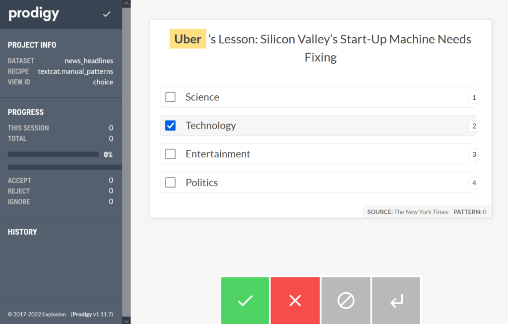
Prodigy is a great tool for annotating the datasets needed to train machine learning models. It has built in support for many kinds of tasks, from text classification, to named entity recognition and even for image and audio annotation.
One of the cool things about Prodigy is that it integrates with Spacy (they are created by the same company), so you can use active learning (having a model suggest annotations and then being corrected by humans) or you can leverage Spacy patterns to automatically suggest annotations.
Prodigy has various recipes for these things, but it doesn’t come with a recipe to use only patterns for manual annotation for a multilabel text classification problem, only in combination with an active learning loop. The problem is that for multi-label annotation, Prodigy does binary annotation for each document, meaning the human annotator will be shown only one label at a time and they’ll have to decide if it’s relevant to the document or not. If you have many labels, it means each document might be shown as many times as there are labels.
I recently had to solve a problem where I knew that most of the documents would have a single label, but in a few cases there would be multiple labels. I also had some pretty good patterns to help bootstrap the process, so I wrote a custom recipe that used only patterns for a multilabel text classification problem.
Code for custom recipe
To do this, I combined some code from the recipes that are provided by Prodigy for text categorization. Let’s see how it work.
First, let’s define the CLI arguments in a file called manual_patterns.py. We’ll need:
@recipe(
    "textcat.manual_patterns",  # Name of the recipe
    dataset=("Dataset to save annotations to", "positional", None, str),
    source=("File path with data to annotate", "positional", None, str),
    spacy_model=("Loadable spaCy pipeline or blank:lang (e.g. blank:en)", "positional", None, str),
    labels=("Comma-separated label(s) to annotate or text file with one label per line", "option", "l", get_labels),
    patterns=("Path to match patterns file", "option", "pt", str),
)
Then we need to define the function that loads the stream of data, runs the PhraseMatcher on it and returns the project config:
The last bit is the function which takes the suggestions generated by the PhraseMatcher and adds them to be selected by default in the UI. In this way, the annotators can quickly accept them:
def add_suggestions(stream, matcher, labels):
    texts = (eg for score, eg in matcher(stream))
    options = [{"id": label, "text": label} for label in labels]

    for eg in texts:
        task = copy.deepcopy(eg)

        task["options"] = options
        if 'label' in task:
            task["accept"] = [task['label']]
            del task['label']
        yield task
Expected file formats
Now let’s run the recipe. Assuming we have an news_headlines.jsonl file in the following format:
{"text":"Pearl Automation, Founded by Apple Veterans, Shuts Down"}
{"text":"Silicon Valley Investors Flexed Their Muscles in Uber Fight"}
{"text":"Uber is a Creature of an Industry Struggling to Grow Up"}
{"text": "Brad Pitt is divorcing Angelina Jolie"}
{"text": "Physicists discover new exotic particle"}
> python -m prodigy textcat.manual_patterns news_headlines news_headlines.jsonl  blank:en --label "Science,Technology,Entertainment,Politics" --patterns patterns.jsonl -F .\manual_patterns.py

Using 4 label(s): Science, Technology, Entertainment, Politics
Added dataset news_headlines to database SQLite.
D:\Work\staa\prodigy_models\manual_patterns.py:67: UserWarning: [W036] The component 'matcher' does not have any patterns defined.
  texts = (eg for score, eg in matcher(stream))

✨  Starting the web server at http://localhost:8080 ...
Open the app in your browser and start annotating!
BERT1Bidirectional Encoder Representations (and it’s numerous variants) models have taken the natural language processing field by storm ever since they came out and have been used to establish state of the art results in pretty much all imaginable tasks, including text analysis.
I am a Christian, so the Bible is important to me. So, I became curious to see what BERT would “think” about the Bible. The manuscripts of the Bible on which modern translations are based were written in Hebrew (Old Testament) and Greek (New Testament). There are many difficult challenges in the translation, resulting in many debates about the meaning of some words. I will conduct two experiments on the text of the New Testament to see what BERT outputs about the various forms of “love” and about the distinction between “soul” and “spirit”.
Quick BERT primer
There are many good explanations of how BERTworks and how it’s trained, so I won’t go into that, I just want to highlight two facts about it:
one of the main tasks that is used to train a BERT model is to predict a word2actually a byte pair encoded token given it’s context: “Today is a [MASK] day”. In this case it would have to predict the fourth word and possible options are “beautiful”, “rainy”, “sad” and so on.
one of the things that BERT does really well is to create contextual word embeddings. Word embeddings are mathematical representations of words, more precisely they are high dimensional vectors (768 in the case of BERT), that have a sort of semantic meaning. What this means is that the word embedding similar words is close to each other, for example, the embeddings for “king”, “queen” and “prince” would be close to each other, because they are all related to royalty, even though they have no common lemma. The contextual part means there is no one fixed word embedding for a given word (such as older models like word2vec or GloVe had), but it depends on the sentence where the word is used, so the word embedding for “bank” is different in the sentence “I am going to the bank to deposit some money” than in the sentence “He is sitting on the river bank fishing”, because they refer to different concepts (financial institution versus piece of land).
Obtaining the embeddings
Reading the data
First, let’s read the Bible in Python. I’ve used the American King James Version translation, because it uses modern words and it’s available in an easy to parse text file, where the verse number (Matthew 15:1) is separated from the text of the verse by a tab (\t):
Genesis 1:1 In the beginning God created the heaven and the earth.
verses = {}
with open('akjv.txt', 'r', encoding='utf8') as f:
    lines = f.readlines()
    for line in lines[23146:]:   # The New Testament starts at line 23146
        citation, raw_sentence = line.strip().split('\t')
        verses[citation] = raw_sentence
The next thing we need is the Strong’s numbers, which are a code for each Greek word (or rather base lemma) that appears in the New Testament. I have found a mapping to tell me the corresponding Strong’s number for (most) English words only for the ESV3I had to rename the New Testament book names and convert the file to UTF8 without BOM translation, which might mean that there are slight differences in verse boundaries, but I don’t think that the words I’m going to be analyzing will be different. Here the format is also verse number, followed by xx=<yyyy> pairs, where xx is the ordinal number for a word in the ESV translation and yyyy is the corresponding Strong’s number.
Matthew 1:1 02=<0976> 05=<1078> 07=<2424> 08=<5547> 10=<5207> 12=<1138> 14=<5207> 16=<0011>
This line says that in Matthew 1:1 the second word in the ESV translation corresponds to the Greek word with Strong’s number 976, the fifth word in English to the word with Strong’s number 1078 and so on. The Strong’s numbers are nicely preformatted into 4 character strings, so we check if a Strong’s number is in a verse by simply looking if the number is in this string, without having to parse each verse.
strongs_tags = {}
with open("esv_tags.txt") as f:
    lines = f.readlines()
    for line in lines:
        verse, strongs = line.split("\t", maxsplit=1)
        strongs_tags[verse] = strongs
Getting the embedding for a word with BERT
Let’s load the BERT model and it’s corresponding tokenizer, using the HuggingFace library:
from transformers import AutoTokenizer, AutoModel

tokenizer = AutoTokenizer.from_pretrained('bert-base-cased')
model = model = AutoModel.from_pretrained('bert-base-cased', output_hidden_states=True).eval()
BERT has a separate tokenizer because it doesn’t work on characters or on words directly, but it works on byte pair encoded tokens. For more frequent words, there is a 1:1 mapping of word – token, but rarer words (or words with typos) will be split up into multiple tokens. Let’s see this for the word “love” and for “aardvark”:
[CLS] and [SEP] are two special tokens, mostly relevant during training. The word_ids function returns the index of the word to which that token belongs. Let’s see an example with a rare word:
In this case, aardvarks (the second word) is split up into 4 tokens, which is why it shows up 4 times in the list obtained from word_ids.
Now, let’s find the index of the word we are looking for in a verse:
def get_word_idx(sent: str,  word: str):
    l = re.split('([ .,!?:;""()\'-])', sent)
    l = [x for x in l if x != " " and x != ""]
    return l.index(word)
We split on punctuation and spaces, skip empty strings and ones with a space and get the index of the word we are looking for.
Because the BPE encoding can give multiple tokens for one word, we have to get all the tokens that correspond to it:
encoded = tokenizer.encode_plus(sent, return_tensors="pt")

idx = get_word_idx(sent, word)
# get all token idxs that belong to the word of interest
token_ids_word = np.where(np.array(encoded.word_ids()) == idx)
In BERT, the best word embeddings have been obtained by taking the sum of the last 4 layers. We pass the encoded sentence through the model to get the outputs at the last 4 ones, sum them up layerwise and then average the outputs corresponding to the tokens that are part of our word:
def get_embedding(tokenizer, model, sent, word, layers=None):
    layers = [-4, -3, -2, -1] if layers is None else layers

    encoded = tokenizer.encode_plus(sent, return_tensors="pt")

    idx = get_word_idx(sent, word)
    # get all token idxs that belong to the word of interest
    token_ids_word = np.where(np.array(encoded.word_ids()) == idx)

    with torch.no_grad():
        output = model(**encoded)

    # Get all hidden states
    states = output.hidden_states
    # Stack and sum all requested layers
    output = torch.stack([states[i] for i in layers]).sum(0).squeeze()
    # Only select the tokens that constitute the requested word
    word_tokens_output = output[token_ids_word]

    return word_tokens_output.mean(dim=0)
Processing the New Testament with BERT
Now let’s get the embeddings for the target words from all the verses of the New Testament. We will go through all the verses and if any of the Strong’s numbers appear in the verse, we will start looking for a variation of the target word in English and get the embedding for it. The embedding, the verse text, the Greek word and the book where it appears will be appended to a list.
def get_all_embeddings(greek_words, english_words):
    embeddings = []

    for key, t in verses.items():
        strongs = strongs_tags[key]
        for word in greek_words:
            for number in greek_words[word]:
                if number in strongs:
                    gw = word

                    for v in english_words:
                        try:
                            if v in t:
                                emb = get_embedding(tokenizer, model, t, v).numpy()
                                book = books.index(key[:key.index(" ", 4)])
                                embeddings.append((emb, f"{key} {t}",  gw, book))
                                break
                        except ValueError as e:
                            print("Embedding not found", t)
                    else:
                        print("English word not found", key, t)
    return embeddings
Next, I am going to take all the verses where one of these target words appear in the New Testament. I am going to mask out their appearance and ask BERT to predict what word should be there.
def mask_and_predict(word_list):
    predictions = []
    for key, t in verses.items():
        for v in word_list:
                if v in t:
                    try:
                        new_t = re.sub(f"\\b{v}\\b", "[MASK]", t)
                        top_preds = unmasker(new_t)
                        if type(top_preds[0]) == list:
                            top_preds = top_preds[0]
                        predictions.append((f"{key} {t}",  v, top_preds))
                        break
                    except Exception:
                        print(new_t, v)
    return predictions
Love
In Greek, there are several words that are commonly translated as love: agape, eros, philia, storge, philautia, xenia, each having a different focus/source. In the New Testament, two of these are used: agape and philia. There is much debate between Christians about the exact meaning of these two words, such as whether agape is bigger than philia, the two are mostly synonyms, or philia is the bigger love.
To try to understand what BERT thinks about these two variants, I am going to extract the 768 dimensional word embeddings for the English word love, reduce their dimensionality with UMAP and plot the results, color coding them by the original word used in Greek.
Now we’ll need the Strong’s numbers for the two words we’re investigating. I included several variations for each word, such as verbs/nouns, or composite variants, such as 5365 – philarguria, which is philos + arguria, meaning love of money.
There are some weird failure cases: in 1 Corinthians 13, famously called the chapter of love, the AKJV uses charity for example instead of love for the Greek word “agape”. I chose to not look for charity as well, so all those uses of “agape” are left out.
Now that we have all the embeddings, let’s reduce their dimensionality with UMAP and then visualize them. They will be color coded according to the Greek word and on hover they will show the verse.
The blue dots are where the Greek is agape (or it’s derivatives), while the red ones are where the Greek is philos.
You can notice 4 clusters in the data. The top right cluster is mostly made out of love that is between Christians. The bottom right one seems to be mostly about the love of God, with the love of money throw in there as well (the blue dot on the right). The cluster on the left seems to be less well defined, with the top side looking like it’s about commandments related to love (you shall love, should love, if anyone will love) and it’s consequences. The bottom left side is the most fuzzy, but I think it seems to be about the practical love of Jesus for humans.
What is easier to notice is that the Greek words agape and philos are mixed together. The love of God cluster (bottom right) seems to be the only one that is agape only (if we exclude the love of money verse, which reeaaaally doesn’t belong with the others), with the exception of the Titus 3:4 verse, which however does sound very much like the others.
However, we can plot the same graph, but this time color coding with the parts of the New Testament where the verse is found:
There is lots of mixing in all clusters, but it seems to me that the Pauline letters use love in a different way then the gospels.
Conclusion? Yes, the word agape does sometimes refer to the love of God, in a seemingly special way, but it often refers to other kinds of love as well, in a way which BERT can’t really distinguish from philos love.
Soul and spirit
The Bible uses two words for the immaterial parts of man: soul (Hebrew: nephesh, Greek: psuche) and spirit (Hebrew: ruach, Greek: pneuma). Again, there is great debate whether the two are used interchangeably or whether they are two distinct components of humans.
After getting the embeddings for these two words, I will plot them as we did before. We can discover quite a few clusters in this way.
In this case, the clusters are almost perfectly separated, with very little mixing. What little mixing happens is usually because in one verse both words occur. Contrast this with the case for agape/phileo, where there is a lot of mixing.
The top right cluster is about the Spirit of God. The one below is about unclean/evil spirits. The middle cluster is about the Holy Spirit. The bottom left cluster is mostly about the spirit of man, with some examples from the other clusters.
The interesting thing is that the two verses used as most common arguments for the soul being distinct from the spirit (1 Thessalonians 5:23 and Hebrews 4:12) are placed in the blue cluster, and they are right next to Matthew 22:37, Mark 12:30 and Luke 10:27, verses which indicate that man is made of different components (heart, soul, mind, strength).
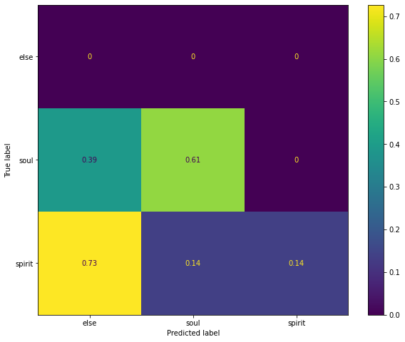
Now, let’s mask out the words soul and spirit and ask BERT to predict the missing word. If BERT mixes the two half the time, it means it thinks there is no distinction between them. Otherwise, they are probably distinct. The resulting confusion matrix:
The y axis represent the true word (soul or spirit), the x axis represents the predicted word (something else, soul or spirit). We can see that in more that 60% of the cases it predicts soul correctly. It never mispredicts it to spirit, but in 40% of the cases it does predict something else. For spirit, the results are worse: it predicts something else quite often, and on top of that, it predicts 50-50% between soul and spirit, so it mixes them up quite often.
The conclusion? The evidence is mixed: on one hand, usages of soul and spirit seem to be mostly different, because they cluster very neatly. But some key verses for the distinction are put in the soul cluster. Now, this might happen because of the way BERT extracts embeddings, two words that are in the same sentence will have similar embeddings. On the other hand, because of the way spirit is mispredicted, it would seem to indicate that there is significant overlap between spirit and soul, at least as “understood” by BERT.
Conclusion
I believe with some polish, BERT-style models can eventually make their way into the toolbox of someone who studies the Bible. They can offer a more consistent perspective to analyzing the text. And of course, they can be used not just to analyze the Bible, but for many other purposes, such as building tools for thoughts (using computers to help us think better and faster), or to analyze all kinds of documents, to cluster them, to extract information from them or to categorize them.
If you need help with that, feel free to reach out to me.
The full code for this analysis can be found in this Colab.
Text classification is a very frequent use case for machine learning (ML) and natural language processing (NLP). It’s used for things like spam detection in emails, sentiment analysis for social media posts, or intent detection in chat bots.
In this series I am going to compare several libraries that can be used to train text classification models.
The fastText library
fastText is a tool from Facebook made specifically for efficient text classification. It’s written in C++ and optimized for multi-core training, so it’s very fast, being able to process hundreds of thousands of words per second per core. It’s very straightforward to use, either as a Python library or through a CLI tool.
Despite using an older machine learning model (a neural network architecture from 2016), fastText is still very competitive and provides an excellent baseline. If you also take into account resource usage, it will be all but impossible to improve on the fastText results, considering that the only models that perform better require powerful GPUs.
Getting started with text classification with fastText
fastText requires the training data for text classification to be in a special format: each document should be on a single line and the labels should be at the start of the line, with the prefix __label__, like this:
Training data format
__label__sauce __label__cheese How much does potato starch affect a cheese sauce recipe?
 __label__food-safety __label__acidity Dangerous pathogens capable of growing in acidic environments
 __label__cast-iron __label__stove How do I cover up the white spots on my cast iron stove?
If you use Doccano for annotating the text data, it has an option to export the data in fastText format. But even if you used another tool for annotation, it’s only a couple of lines of Python code to convert to the appropriate format. Let’s say we have our data in a JSONL format, with each JSON object having a labels key and a text key. To convert to fastText format, we can use the following short snippet:
with open("fasttext.txt", "w") as output:
    with open("dataset.jsonl", encoding="utf8") as f:
        for l in f:
            doc = json.loads(l)
            labels = [x.replace(" ", "_") for x in doc['labels']]
            labels = " ".join(f"__label__{x}" for x in labels)
            txt = " ".join(l['text'].splitlines())
            line = f"{labels} {txt}\n"
            output.write(line)
Training text classification models with fastText
After you have the data in the right format, the simplest way to use fastText is through it’s CLI tool. After you installed it, you can train a model with the supervised subcommand:
> ./fasttext supervised -input fasttext.txt -output model
Read 0M words
Number of words:  16568
Number of labels: 736
Progress: 100.0% words/sec/thread:   47065 lr:  0.000000 avg.loss: 10.027837 ETA:   0h 0m 0s
You can evaluate the model on a separate dataset with the test subcommand and you will get the precision and recall for the first candidate label:
> ./fasttext test model.bin validation.txt
N       15404
P@1     0.162
R@1     0.0701
You can also get predictions for new documents:
> ./fasttext predict model.bin -
How to make lasagna?
__label__baking
Best way to chop meat
__label__food-safety
How to store steak
__label__food-safety
fastText comes with a builtin hyperparameter optimizer, to find the best model on a validation dataset, within the given time (5 minutes by default):
> ./fasttext supervised -input fasttext.txt -output model -autotune-validation validation.txt
If we reevaluate this model we’ll find it performs much better:
> ./fasttext test model.bin validation.txt
N       15404
P@1     0.727
R@1     0.315
A precision of 0.72, compared to 0.16 before. Not bad, for 10 minutes of our time, out of which 5 was waiting for the computer to find us a better model1Autotuning and performance evaluation should happen on separate datasets, to avoid overfitting, so real world performance is likely a bit worse than we got here.
Optimizing for different metrics
This library provides a couple of knobs you can use to try to obtain better models, from what kind of n-grams to use, how big the learning rate should be, what should be the loss function, but also what metric are you trying to optimize. Is precision or recall better aligned with your business KPIs? Is it more important to have the top result be a really good one or are you looking for several good results among in the top 5? Are you only interested in high confidence results? All this depends on the problem you are trying to solve and fastText provides ways to optimize for each of those.
Cons of fastText
Of course, fastText has some disadvantages:
Not much flexibility – only one neural network architecture from 2016 implemented with very few parameters to tune
No option to speed up using GPU
Can be used only for text classification and word embeddings
Doesn’t have too wide support in other tools (for deployments for example)
Conclusion
fastText is a great library to use when you want to start solving a text classification problem. In less than half an hour, you can get a good baseline going, which will tell you if this is a problem that is worth pursuing or not.