|
Your AI feature works. Prove it.
Machine Learning Consulting
|
|
|
|
|
|
The AI coding space is moving at an uncomfortable pace. Even as an AI consultant who tracks this full time, I can’t keep up with every tool that launches. Today’s best model is from Anthropic. Next week it might be OpenAI. The week after, Google surprises everyone. This is a challenge for large companies, because they are used to more stability. But here are some things they have too look at when making decisions in this space: 1. The modelAnthropic has the Claude series, OpenAI has GPT, Google has Gemini. Each family gets meaningful updates every few months, and which one leads on any given benchmark shifts constantly. More importantly, models aren’t uniformly good. Some are better at generating new code, some at finding bugs, some at reasoning through long-running autonomous tasks. This usually reflects where that company focused its training efforts in the last cycle — which means the rankings shift as priorities shift. Don’t pick a model based on a benchmark from three months ago. 2. The harnessThe harness is how your team actually interacts with the model — an IDE integration, a terminal agent, a chat interface. This matters more than most people realise. Anthropic’s models have been specifically optimised for use inside Claude Code, and they perform measurably better there than when accessed through a generic wrapper. Other models are trained more broadly and don’t have a preferred harness. Some harnesses give models access to more tools — not just file editing, terminal execution, web search — and this directly affects what they can accomplish on real tasks. The practical implication: if your team builds workflows, hooks and institutional knowledge around a specific harness, that investment doesn’t transfer easily. Lock-in at the harness level is just as big of a risk as lock-in at the model level. 3. Infrastructure and data residencyWhere is the model running, and where is your data going? Claude is available directly through the Anthropic API and through all major cloud providers. Gemini is Google-only. Some APIs let you specify that requests stay in Europe — important for GDPR compliance. Others route to wherever spare capacity exists, with no guarantees. For regulated industries or anything involving sensitive data, this is the first requirement that needs to be met, not an afterthought. 4. Payment modelThere are three main payment models: Subscription gives you predictable costs but unpredictable performance. Providers have a perverse incentive to quietly degrade quality during peak periods, either by serving a quantized model, or by changing the default thinking budget. Subscription pricing is also heavily subsidised right now. When that subsidy has to give way to sustainable unit economics, the price will look very different. Per-request pricing, as used in GitHub Copilot, is conceptually tidy but practically broken. Requests vary enormously in complexity. Pricing them uniformly means either the provider loses money on hard tasks or you overpay on easy ones. I don’t see this surviving long-term. Token-based pricing — you pay for exactly what you use — is the most transparent and the most portable. It gives you access to any harness, any model, through APIs or aggregators like OpenRouter. It’s also the most expensive one (Uber went through their whole budget for 2026 in just Q1), but many companies find that it still gives them a very good ROI. The practical adviceDon’t make a five-year platform decision in a market that changes every five months. Run experiments across different teams, don’t sign contracts that are hard to exit, and plan explicitly to revisit the decision every six months. Build that review cadence into the rollout, not as an afterthought. Next issue I’ll cover the questions this one doesn’t answer: security and legal vetting, the lock-in risk in more depth, and when local models actually make sense for enterprise teams. Is your team navigating any of these decisions right now? Hit reply — I’m curious what’s causing the most friction. |
How I Write Software with LLMsOver the last year I’ve written more than 100,000 lines of code using AI. I’ve landed on a workflow I’m genuinely happy with — both in how it feels to use and in the quality of the resulting code. Most people I see either give a vague prompt, get a disappointing result, and give up — or go the other direction and build complex orchestration pipelines with a dozen moving parts that are too unreliable to trust. This is what works for me in between those two extremes. The toolsMy main driver is Claude Code with Opus, unless the task is small (roughly under 100 lines), in which case Sonnet is fine. For a second opinion and for certain tasks, I use OpenAI’s Codex on GPT-5.4 at xhigh reasoning. Using two models deliberately isn’t redundancy — they have different personalities and catch different things. Start with clarification, not codeWhenever I start a new session, I describe what I want — the rough feature outline, what’s in my head — and then I explicitly tell the model to ask me questions about anything unclear. This step is non-negotiable. Skip it and the model will silently make a guess at every ambiguous decision. Run it again and it’ll make different guesses. You’ll get code that works but isn’t quite what you wanted, and you won’t immediately know why. I iterate on this — asking for more questions several times — until both of us feel like the specification is nailed down. The more precise the spec, the more mechanical the code generation becomes. That’s the goal. Planning large featuresFor anything substantial — a new section of the app, a significant new feature — I use plan mode. The model reads through the codebase, identifies existing patterns, and produces a detailed plan before writing a single line of code. Claude’s plans tend to be very explicit: endpoints, data shapes, what gets touched and why. Once I have that plan, I pass it to Codex and ask it to critique. Codex is more nitpicky and tends to catch smaller issues Claude glosses over. I take those suggestions back to Claude, do a few revisions, and only once everyone agrees does Claude write the actual code. Reviewing the outputI don’t read every line — that’s not realistic at scale. Instead I take a high-level pass at which files were touched. This alone catches a surprising number of mistakes: code that didn’t reuse something already written, or changes that introduced cross-module dependencies that shouldn’t exist. If anything looks off, I flag it immediately. Then I send the code to a different model for review — if Opus wrote it, Codex reviews it. Or I open a pull request on GitHub and let whatever review tool is set up on that project do its pass. DebuggingFor gnarly bugs — not new features, but things that are genuinely broken and require real digging — GPT-5.4 on xhigh is my first call. It’s persistent in trying different approaches and has a noticeably high hit rate on hard problems. The part most people skipAll of this only works because of the upfront specification work. The cool thing is that you can stress-test a spec from every angle before writing any code — ask the model to rewrite it from a different perspective, challenge your assumptions, find edge cases. This costs almost nothing. And once the spec is solid, turning it into working code is almost trivially easy by comparison. I could automate more — trigger reviews automatically, chain agents together, remove myself from the loop. I’ve chosen not to. Manual review checkpoints mean I still understand what’s being built. That matters to me both as an engineer and when I’m explaining these workflows to teams. What does your workflow look like? Reply and let me know — I’m especially curious whether anyone has found a reliable way to do the spec phase without going back and forth as many times as I do. |
|
What will the future software engineer do? |
|
GitHub Copilot vs Cursor vs… GitHub Copilot was the first tool to use AI to help with coding, back in the smart autocomplete era. It took me a while to start using it — how can a machine write code better than me? But after a friend strongly recommended it, I fell in love with it. Then other competitors started appearing. They kept adding new features to Copilot, but spread themselves too thin — too many weird features (look for the sparkle button in random places and try to guess what it does). As a result, they didn’t do any one thing particularly well. It also took them a looong time to add a CLI interface. AIDER was one of those early tools. It was the first CLI AI tool. It was clunky — models were not as good back then. But it showed the first signs of being able to do autonomous edits. It got things working, but the code quality wasn’t the best. And being first in a domain comes with a cost — they were stuck with architectural choices that didn’t scale well, eventually lost relevance, and development stopped. At some point, Cursor became the highly favored startup. It works really well — but it required using their IDE. Back then, AI agents were not good enough to replace an IDE, and for Python, nothing beats PyCharm. Then Claude Code appeared. I remember blowing $15 in a couple of hours using it. Initially, it felt like a slot machine — will I get good code this time? But what kept me using Claude Code is the strong integration between the model and the environment. Anthropic builds both, so Claude models work best there, because they’re trained to use it. The same model in another app performs slightly worse. I also use Codex (mostly when I run out of my Claude subscription). It’s pretty good, but it has a colder personality, so I don’t enjoy it as much. I’ve tried Google’s tools too. First off, Gemini has a somewhat depressive personality (if it keeps failing at a task, it might say it will delete itself — https://www.forbes.com/sites/lesliekatz/2025/08/08/google-fixing-bug-that-makes-gemini-ai-call-itself-disgrace-to-planet/). And Antigravity (their IDE) is an example of poor vibe coding. Unusable. What about you — which AI coding tools have you actually found useful so far? |

A while go someone asked me some questions about Qdrant and how to optimize it’s usage for use case that they were having separate document sets for each “client”. When doing searches, they wanted to search only the documents belonging to the client doing the search.
One of the things that we discussed was whether it’s better to have a single collection for all documents and use a field “client_id” for filtering the results, or to use a separate collection for each client.
So I wrote a quick benchmark for this (with my friend Claude of course) to compare these scenarios. In the case of single collection, I tested both without an index and with a keyword index on the “client_id” field.
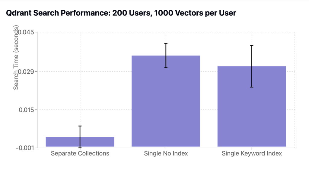
| Configuration | Search Time (ms) | Standard Deviation (ms) |
|---|---|---|
| Separate Collections | 3.8 | 4.3 |
| Single Collection (no index) | 35.8 | 4.8 |
| Single Collection (keyword index) | 31.6 | 8.2 |
Turns out using separate collections is much faster and this holds even for much larger values of users (I tested up to 2000).
Why could that be?
Of course this isn’t a very comprehensive benchmark. There are many other options you can try out, such as the quite recently introduced tenant index. And having things in a single collection has some other advantages, including some operational ones. Reach out to me if you need help with managing Qdrant for your RAG use cases.
You can find the code to reproduce this in this repo.